1. Why Integrate SFT and RL?
While Reinforcement Learning can effectively enhance a model’s reasoning capabilities, a crucial prerequisite is that the base model already possesses some degree of the relevant abilities. In RL training, further improvement is only possible if the model can sample correct trajectories through multiple rollouts. This undoubtedly limits the exploration space of RL.
Therefore, the mainstream approach is to first equip the model with foundational abilities via SFT, and then leverage RL to further enhance these capabilities. However, some studies argue that this two-stage approach is not optimal:
[1] found through experiments that RL improves performance on low-to-medium difficulty problems, while SFT is more effective for high-difficulty problems.
[4] argues that SFT data constructed by larger models(or experts) contains logic leaps that are difficult to imitate through SFT alone. This make it challenging to rollout effective positive samples during the subsequent RL phase.
[3] and [5] directly assert that two separate stage are unnecessary and should be unified.
[6] provides further analysis, finding a kind of adversarial tension between SFT and RL: SFT pushes the model to deviate significantly from the base model, while RL pulls it back to the base model.
In summary, these studies all point to the necessity of merging SFT and RL into a single stage.
2. Background Knowledge
The standard LLM training pipeline typically consists of three stages: Pre-training, SFT and RL. The Pre-training stage uses an autoregressive objective to train model on a massive dataset, laying the foundation for the subsequent Post-training phase. Post-training is usually divided into SFT and RL, both of which require a diverse set of prompts $\mathcal{D}$.
2.1 SFT
In this stage, for a prompt $x\sim\mathcal{D}$, a high-quality response $y$ is constructed through methods like expert writing, manual synthesis, or distillation from a stronger model. Let’s assume $y\sim\pi_{\phi}(\cdot|x)$, where $\pi_{\phi}$ represents the policy of the human expert or a stronger model. Then, the loss function of SFT training is:
$$ L_{\text{SFT}}=-\mathbb{E}_{x\sim D,y\sim\pi_\phi(\cdot|x)}\left[\log\pi_{\theta}(y|x)\right]=-\mathbb{E}_{x\sim D,y\sim\pi_\phi(\cdot|x)}\left[\sum_{t=1}^{|y|}\log\pi_{\theta}(y_t|x,y_{\le t})\right] \quad (1) $$The gradient of this loss function is expressed as:
$$ \nabla_{\theta} L_{\text{SFT}}=-\mathbb{E}_{x\sim D,y\sim\pi_\phi(\cdot|x)}\left[\nabla_{\theta}\log\pi_{\theta}(y|x)\right]=-\mathbb{E}_{x\sim D,y\sim\pi_\phi(\cdot|x)}\left[\sum_{t=1}^{|y|}\nabla_{\theta}\log\pi_{\theta}(y_t|x,y_{\lt t})\right] \quad (2) $$2.2 RL
RL is typically performed after the SFT stage. In an on-policy setting, for a prompt $x\sim\mathcal{D}$, a response $y$ is sampled from the current policy $\pi_{\theta}$. The loss function of RL is:
$$ L_{\text{RL}}=-\mathbb{E}_{x\sim D,y\sim\pi_{\theta}(\cdot|x)}\left[R(x,y)\right] \quad (3) $$The policy gradient for this loss function is:
$$ \nabla_{\theta}L_{\text{RL}}=-\mathbb{E}_{x\sim D,y\sim\pi_{\theta}(\cdot|x)}[R(x,y)\nabla_{\theta}\log\pi_{\theta}(y|x)]=-\mathbb{E}_{x\sim D,y\sim\pi_{\theta}(\cdot|x)}\left[\sum_{t=1}^{|y|}R_t\nabla_{\theta}\log\pi_{\theta}(y_t|x,y_{\lt t})\right] \quad (4) $$Here, $R_t$ is the reward for the partial sequence $(x,y_{\lt t})$. Equation (4) represents the standard REINFORCE gradient. In practice, to reduce variance, REINFORCE with a baseline is often employed. REINFORCE with a baseline essentially replaces the reward with an advantage function. Compared to the reward’s absolute value, the advantage function represents the degree of improvement over a baseline. Therefore, the gradient for REINFORCE with a baseline is:
$$ \nabla_{\theta}L_{\text{RL}}=-\mathbb{E}_{x\sim D,y\sim\pi_{\theta}(\cdot|x)}\left[\sum_{t=1}^{|y|}A_t\nabla_{\theta}\log\pi_{\theta}(y_t|x,y_{\lt t})\right]\quad(5) $$where $A_t$ is the advantage of $(x,y_{\lt t})$.
2.2.1 GRPO
GRPO has become the de facto standard for RL algorithms in LLM post-training. GRPO is a critic-free variant of PPO. For a give prompt $x$, it samples $G$ response, denoted as $\lbrace y_i\rbrace_{i=1}^G$, where each response $y_i$ is associated with a scalar reward $R_i$. While standard PPO requires a critic model to help compute advantage, GRPO approximates the advantage using in-batch normalization:
$$ A_{i,t}=\frac{R_i-\text{mean}([R_1,\dots,R_G])}{\text{std}([R_1,\dots,R_G])} \quad(6) $$Here, $A_{i,t}$ represents the advantage for the $t$-th token of the $i$-th response. Apart from this method of advantage calculation, its loss function is similar to that of PPO:
$$ L_{\text{GRPO}}=-\mathbb{E}_{x\sim D,\lbrace y_i\rbrace_{i=1}^G\sim\pi_{\theta_{\text{old}}}(\cdot|x)}\left[\frac{1}{G}\sum_{i=1}^G\frac{1}{|y_i|}\sum_{t=1}^{|y_i|}\min\left(r_{i,t}(\theta)A_{i,t},\text{clip}(r_{i,t}(\theta),1-\varepsilon,1+\varepsilon)A_{i,t}\right)\right] \quad (7) $$where $r_{i,t}(\theta)=\frac{\pi_{\theta}(y_t|x,y_{\lt t})}{\pi_{\theta_{\text{old}}}(y_t|x,y_{\lt t})}$ is the importance sampling ratio.
3. Alternating SFT and RL
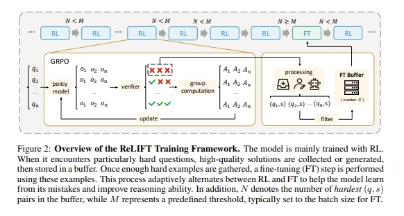
ReLIFT[1] suggests that RL improves performance on low-to-medium difficulty problems, while SFT is more effective for high-difficulty problems. Therefore, it proposes an alternating scheme. Specifically, during the RL stage, samples from rollouts that are entirely incorrect are placed into a buffer pool. When the buffer pool is full, SFT is performed on these samples.
4. Using SFT as Off-Policy samples for RL
Instead of alternating SFT and RL, LUFFY[2] treats SFT data as off-policy samples and integrates them into the RL process through importance sampling. This is a more natural approach.
4.1 Notation
- $D_{on}=\lbrace(x,y_i)|y_i\sim\pi_{\theta_{\text{old}}}(\cdot|x),i=1,\dots,N_{on}\rbrace$ represents the $N_{on}$ trajectories obtained by rolling out directly from the policy.
- $D_{off}=\lbrace(x,y_i^*)|y_i^*\sim\pi_\phi(\cdot|x),i=1,\dots,N_{off}\rbrace$ represents the $N_{off}$ SFT data points.
- $\text{CLIP}(r_{i,t}(\theta), A_{i,t},\varepsilon)=\min\left(r_{i,t}(\theta)A_{i,t},\text{clip}(r_{i,t}(\theta),1-\varepsilon,1+\varepsilon)A_{i,t}\right)$.
4.2 Mixing On- and Off-Policy Samples
The most straightforward method is directly mix the off-policy samples with the on-policy data for training. The loss function can then be written as:
$$ L_{\text{naive\_mix}}=-\frac{1}{Z}\left[\underbrace{\sum_{j=1}^{N_{off}}\sum_{t=1}^{|y_j^*|}\text{CLIP}(r_{j,t}(\theta),A_{j,t},\varepsilon)}_{\text{off policy objective}}+\underbrace{\sum_{i=1}^{N_{on}}\sum_{t=1}^{|y_i|}\text{CLIP}(r_{i,t}(\theta),A_{i,t},\varepsilon)}_{\text{on policy objective}}\right] \quad (8) $$where $Z=\sum_{j=1}^{N_{off}}|y_j^*|+\sum_{i=1}^{N_{on}}|y_i|$ is the normalization factor.
However, using $r_{j,t}(\theta)=\frac{\pi_{\theta}(y_{j,t}|x,y_{j,\lt t})}{\pi_{\theta_{\text{old}}}(y_{j,t}|x,y_{j,\lt t})}$ for the importance sampling ratio in the off-policy objective is not appropriate, because the denominator $\pi_{\theta_{\text{old}}}$ is not the distribution that generated the off-policy data $y_j^*$. Therefore, the first term should use a new importance sampling ratio:
$$ r_{j,t}(\theta,\phi)=\frac{\pi_{\theta}(y_{j,t}|x,y_{j,\lt t})}{\pi_{\phi}(y_{j,t}|x,y_{j,\lt t})}\quad(9) $$Replacing the ratio in Equation (8) with this new importance sampling ratio (9) yields the final mixed loss function:
$$ L_{\text{mix}}=-\frac{1}{Z}\left[\underbrace{\sum_{j=1}^{N_{off}}\sum_{t=1}^{|y_j^*|}\text{CLIP}(r_{j,t}(\theta,\phi),A_{j,t},\varepsilon)}_{\text{off policy objective}}+\underbrace{\sum_{i=1}^{N_{on}}\sum_{t=1}^{|y_i|}\text{CLIP}(r_{i,t}(\theta),A_{i,t},\varepsilon)}_{\text{on policy objective}}\right] \quad (10) $$4.3 Importance Sampling Correction
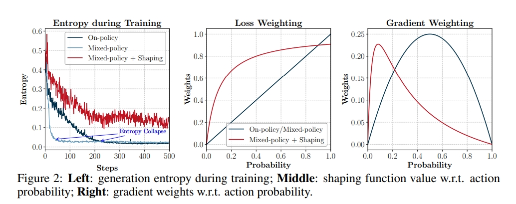
Although training with Equation (10) addresses the gradient bias issue, it was observed to significantly suppress exploration while accelerating convergence, leading to rapid entropy collapse, as shown in the left figure above.
Further analysis suggests that when the model receives both on- and off-policy signals simultaneously, it tends to prioritize reinforcing tokens that have a high probability in both on-policy and off-policy trajectories. Low-probability tokens from off-policy trajectories, which are crucial for reasoning, receive a weak signal because their importance ratio $r_{j,t}(\theta,\phi)$ is too small. Therefore, [2] proposes using correction function $f(x)=\frac{x}{x+\gamma}$ to adjust the importance sampling ratio $r_{j,t}(\theta,\phi)$, i.e., replacing $r_{j,t}(\theta,\phi)$ in Equation (10) with $f(r_{j,t}(\theta,\phi))$.
5. Simultaneous SFT and RL
In contrast to LUFFY[2], which unifies training by treating SFT data as off-policy samples, SRFT[6] takes a practical approach by simultaneously applying both SFT and RL losses.
SFT loss Function. The standard SFT loss function is shown in Equation (1). However, SRFT reasons that if a sample’s entropy is too high, it indicates the sample is unfamiliar to the current model. In this case, the weight of the SFT loss function should be reduced. Therefore, it employs a weighted SFT loss fuction:
$$ L_{\text{SFT}}=-w_{\text{SFT}}\cdot\mathbb{E}_{(x,y)\sim D_{\text{SFT}}}\left[\log\pi_{\theta}(y|x)\right] \quad(11) $$where $w_{SFT} = 0.5 \times \text{stop_grad}(\exp(-H(\pi_\theta)))$.
Off-Policy RL Loss Function. Similar to LUFFY, SFT data is treated as off-policy samples:
$$ L_{\text{RL}}^{off}=-E_{(x,y)\sim D_{SFT}}[\text{CLIP}(r_{i,t}(\theta,\phi), A_{i,t},\varepsilon)] \quad(12) $$where $r_{i,t}(\theta,\phi)$ is the same as in LUFFY’s Equation (9).
On-Policy RL Loss Function. Under a binary reward setting of {+1,-1}, the standard on-policy RL loss function is:
$$ \begin{aligned} L_{\text{RL}}^{on}&=-\mathbb{E}_{x \sim D, y \sim \pi_\theta(\cdot|x)}[R(x,y)\log\pi_\theta(y|x)] \\ &=-\mathbb{E}_{x \sim D, y^+ \sim \pi_\theta(\cdot|x)}[\log\pi_\theta(y^+|x)] + \mathbb{E}_{x \sim D, y^- \sim \pi_\theta(\cdot|x)}[\log\pi_\theta(y^-|x)] \end{aligned} $$However, to mitigate entropy collapse, SRFT adds an entropy-based weight to the loss term for positive samples:
$$ L_{\text{RL}}^{on}=-w_{RL}\cdot\mathbb{E}_{x \sim D, y^+ \sim \pi_\theta(\cdot|x)}[\log\pi_\theta(y^+|x)] + \mathbb{E}_{x \sim D, y^- \sim \pi_\theta(\cdot|x)}[\log\pi_\theta(y^-|x)] \quad(13) $$where $w_{RL} = 0.1 \times \text{stop_grad}(\exp(H(\pi_\theta)))$. When the entropy is high, it means the model is uncertain about the sample, and a larger $w_{RL}$ forces the model to learn more from it.
Final Loss Function. The final loss function is the sum of Equation (11), (12) and (13):
$$ L_{\text{SRFT}}=L_{\text{SFT}}+L_{\text{RL}}^{off}+L_{\text{RL}}^{on}\quad(14) $$Therefore, this method simultaneously performs SFT, Off-Policy RL, and On-Policy RL.
6. Using SFT as Hint
A hint is defined as the concatenation of a problem and a partial correct answer. A key problem with standard RL is its inability to roll out positive samples for difficult problems. SFT data, serving as natural positive samples, can be construct a hint by concatenating a portion of these expert response with the problem statement. The policy then preforms rollouts based on this hint, rather than the original prompt.
Hint-based methods primarily revolve around two questions: a. How to construct a suitable hint? b. How to handle the hint portion during training?
6.1 How to Construct a Suitable Hint
Dynamically Adjusting Hint Length. Both [3] and [5] adopt methods to dynamically adjust hint length, thereby creating hints with progressively increasing difficulty. This approach not only adjusts the difficulty level but also mitigates the train-test discrepancy. Assuming a full SFT sample has length $L$, [3] uses a cosine annealing schedule to dynamically adjust a proportion coefficient $p\in [0,1]$. Instead of directly using $p\cdot L$ as the hint length, it samples a length $l$ from a binomial distribution with $L$ trials and success probability $p$. [5] samples the length from a dynamic interval $U(low,high)$, where the upper bound high is fixed and the lower bound low decays from high to 0 following a cosine schedule. This way, the model gradually transitions from needing a long hint to answer correctly to being able to answer independently.
Adjusting Hints Based on the Rollout Results. [4] proposes a binary search method to find an appropriate hint. The logic is as follows:
- If all rollouts based on the current hit fail, the hint is lengtheded.
- if all rollouts based on the current hit succeed, the hint is shortened.
- if the results are mixed, the hint is considered to be of appropriate difficulty.
6.2 Training Methods
Standard RL Training. Both [4] and [5] treat rollouts generated from hints as standard rollouts and train them using standard RL methods. While [4] uses only hint-based rollouts, [5] mixes standard rollouts with hint-based rollouts for training. Furthermore, [5] argues that directly applying reinforcement learning to the hint part can force the model to learn low-probability tokens, causing large gradients and training instability. Therefore, it proposes filtering the tokens from SFT hint, retaining gradients only for the top-k% of tokens with the highest entropy.
Combined SFT and RL Training. [3] applies different loss functions to the hint and rollout portions of a trajectory. It uses an SFT loss for the hint part and an RL loss for the rollout part. Specifically, in a GRPO setting, each prompt $x$ generates $G$ response $\lbrace y_i\rbrace_{i=1}^G$, where the first $l_i$ tokens of each response $y_i$ constitute the hint. The loss function is then:
$$ L_{\text{UFT}}=-\mathbb{E}_{x,\lbrace y_i\rbrace_{i=1}^G}\frac{1}{G}\sum_{i=1}^G\left[ \underbrace{\frac{1}{|y_i|-l_i}\sum_{t=l_i}^{|y_i|}\min\left(r_{i,t}(\theta)A_{i,t},\text{clip}(r_{i,t}(\theta),1-\varepsilon,1+\varepsilon)A_{i,t}\right)}_{RL} +\underbrace{\beta\sum_{t=0}^{l_i}\log\pi(y_t|x,y_{\lt t})}_{SFT} \right]\quad(15) $$References
[1]. Learning What Reinforcement Learning Can’t: Interleaved Online Fine-Tuning for Hardest Questions
[2]. Learning to Reason under Off-Policy Guidance
[3]. UFT: Unifying Supervised and Reinforcement Fine-Tuning
[4]. BREAD: Branched Rollouts from Expert Anchors Bridge SFT & RL for Reasoning
[5]. Blending Supervised and Reinforcement Fine-Tuning with Prefix Sampling
[6]. SRFT: A Single-Stage Method with Supervised and Reinforcement Fine-Tuning for Reasoning